


- Follow Tarun's Blog on WordPress.com
-
Recent Posts
Categories
Goodreads
Archives
1. Kennedy Space Center (KSC)
")
NASA’s John F Kennedy Space Centre tops the list of must-visit places for techies. Located on Merritt Island, Florida, the center manages and operates America’s astronaut launch facilities.
KSC’s Visitor Complex provides public tours of the center and adjacent Cape Canaveral Air Force Station. The tour’s highpoint is A/B Camera Stop where visitors can access the closest possible Space Shuttle launch pad viewing site.
2. Chicago Museum of Science and Industry

Located in Chicago’s Jackson Park, the Museum of Science and Industry (MSI) has over 2,000 exhibits, displayed across 75 halls.
The Museum features a working coal mine, a German submarine (U-505) captured during World War II, a 3,500-square-foot (330 m2) model railroad, the first diesel-powered streamlined stainless-steel passenger train (Pioneer Zephyr), and a NASA spacecraft used on the Apollo 8 mission.
The museum’s major exhibits include Science Storms, YOU the Experience, Earth Revealed, U-505, Fast Forward and The Smart Home.
3. CERN (European Organization for Nuclear Research)
")
European Organization for Nuclear Research or CERN is one of the hottest hub of scientific research globally. Located astride the Franco-Swiss border near Geneva, CERN is one of the world’s largest and most respected centres for scientific research.
At CERN, the world’s largest and most complex scientific instruments are used to study the basic constituents of matter. By studying what happens when these particles collide, physicists learn about the laws of Nature.
Founded in 1954, the organization has twenty European member states. The place also holds significance as the birthplace of the World Wide Web. In 1990, physicist Tim Berners-Lee and systems engineer Robert Cailliau devised the concept of an information system based on hypertext links.
This is where father of Internet Tim Berners-Lee wrote a proposal for information management showing how information could be transferred easily over the Internet by using hypertext.
4. The Atomium

One of the major attractions in Brussels, this 102-meters (335 ft.) tall monument was built during 1958 Brussels World’s Fair.
The structure has nine steel spheres connected which forms the shape of a unit cell of an iron crystal magnified 165 billion times. Designed by Andre Waterkeyn, the top sphere provides a panoramic view of Brussels. Each sphere is 18 meters in diameter.
Tubes which connect the spheres along the 12 edges of the cube and all eight vertices to the centre enclose escalators connecting the spheres which has exhibit halls and other public spaces.
5. International Spy Museum

The International Spy Museum located in Washington, DC has over 600 artifacts, weapons, bugs, cameras, vehicles, and technologies used for espionage.
The museum houses objects that were supposedly used for spying dating back to Greek, Roman and British empire; American Revolutionary War; and World Wars.
Visitors can also learn about microdots and invisible ink, buttonhole cameras and submarine recording systems.
6. The Computer History Museum

Housing the largest collection of computing artifacts, the Computer History Museum built in 1996 is located in California.
The Museum has three key exhibits: “Mastering the Game,” a history of computer chess; “Innovation in the Valley,” a look at Silicon Valley companies and people; and a Difference Engine designed by Charles Babbage in the 1840s and constructed by the Science Museum.
The place also has rare objects like Cray-1 supercomputer, Cray-2, Cray-3, the Utah teapot, the 1969 Neiman Marcus Kitchen Computer, an Apple I, an example of the first generation of Google’s racks of custom-designed web servers, and the first coin-operated video game
7. Jet Propulsion Laboratory (JPL)
")
Located outside Los Angeles, Jet Propulsion Laboratory’s key function is the construction and operation of robotic planetary spacecraft. The lab also conducts Earth-orbit and astronomy missions.
The lab offers free tours which includes a multimedia presentation on JPL, visits to the Spacecraft Assembly Facility and live demonstrations of JPL science and technology.
The lab also operates NASA’s Deep Space Network
8. German Museum of Technology

Founded in 1982 in Berlin, German Museum of Technology has a large collection of historical technical artifacts. The museum has also recently opened maritime and aviation exhibition halls. It also contains a science center called Spectrum.
The museum houses an array of radios, phones, planes, sea-faring vessels and two whole locomotive sheds.
In the year 2002, the museum opened a special exhibition which featured the inventions of computer pioneer Konrad Zuse.
9. Bletchley Park, England

Best known as the Winston Churchill’s secret intelligence and computers headquarters during World War II, Bletchley Park is also the home town of Milton Keynes. Situated in Buckinghamshire, UK, it is regarded as the site of secret British code breaking activities during World War II and also the birthplace of the modern computer.
In 1939 during the World War II, cryptologists based at Bletchley Park successfully broke major codes used by German military and high command and those of other Axis countries. The most famous break-ins were the ciphers generated by the German Enigma and Lorenz machines. Today, Bletchley Park houses permanent collection of Enigma and other vintage cypher machines and equipment.
It was in Huts 3,6,4 and 8 that the highly effective Enigma decrypt teams worked. The huts operated in pairs and, for security reasons, were known only by their numbers. Their raw material came from the ‘Y’ Stations: a Web of wireless intercept stations dotted around Britain and in a number of countries overseas. These stations listened in to the enemy’s radio messages and sent them to Bletchley Park to be decoded and analyzed
10. Moore School of Engineering, University of Pennsylvania

Regarded as the birthplace of the computer industry, the Moore School is where the first general-purpose digital electronic computer, the ENIAC (Electronic Numerical Integrator And Computer), was built between 1943 and 1946.
ENIAC was capable of being reprogrammed to solve a full range of computing problems. ENIAC was designed to calculate artillery firing tables for the US Army’s Ballistic Research Laboratory, but its first use was in calculations for the hydrogen bomb.
Not only this, the place holds special importance as the first computer course was given at the Moore School in Summer 1946. Also, Moore School faculty John Mauchly and J Presper Eckert founded the first computer company, ENIAC, which produced the UNIVAC computer. The 3-storey Moore School has now been integrated into Penn’s School of Engineering and Applied Science.

AIB headquarters
Allied Irish Banks (AIB) is attempting to recoup around €84 million from Oracle FSS, which was contracted by the bank to supply its core banking software. The bank claims these were the costs and expenditure it ‘wasted’ on trying to implement Oracle FSS’s Flexcube as a retail banking system. AIB is seeking damages for misrepresentation, breach of contract and negligence. It is also claiming further compensation for loss of profits and damage to goodwill, with the amount yet to be calculated. The bank’s action has been transferred to the Commercial Court.
The vendor was originally contracted in 2005 to provide the software for AIB’s wholesale banking activity (to replace Misys’ Bankmaster). At the time, the vendor was known as I-flex Solutions (it was bought by Oracle the same year – IBS, September 2005, Market weighs up Oracle/I-flex deal; and rebranded as Oracle FSS a few years later – IBS, April 2008, I-flex is no more; long live Oracle FSS?).
Flexcube Universal Banking System (UBS) was selected ahead of offerings from Misys and Temenos. Besides Bankmaster, Misys also had an implementation of its Opics system for FX and other dealing operations at AIB and Temenos had an implementation of its T24 banking system at AIB International Financial Services (IBS, February 2009, AIB IFS: Outsourcing on the agenda?). Speaking to IBS in early 2010, AIB’s head of operations and technology, Marcel McCann, said that the decision to go with Flexcube was based not only on functionality but also the ‘capability that we believed the I-flex guys had in helping us to implement it, versus the Temenos guys’ (IBS, February 2010, AIB: When Irish eyes are smiling).
The 2005 Flexcube deal, dubbed Project Pentagon, does not appear to be part of the bank’s action. In the aforementioned IBS interview, McCann stated that Oracle FSS had fulfilled its part of the deal well, and the only rough edges to the project centred on ‘the usual things you’d find on a project of this scale’. ‘But at no stage did we feel that we were up a cul de sac, having made the wrong decision. We wouldn’t change the decision we made or the relationship we have with Oracle FSS because all those things are working very well,’ he said.

Marcel McCann, AIB
However, this agreement gave AIB an option to acquire Oracle FSS’s software for its retail banking activity. This project, known as Project Acorn, was given the green light in 2007 (IBS, May 2007, Who’s bought what?). Prior to signing for Flexcube, the bank evaluated its other existing providers, including Temenos, Misys and SAP (the bank was rolling out SAP’s GL at the time). The final decision came down to Oracle FSS and SAP. In parallel, AIB set about selecting a systems integration partner, ultimately choosing another incumbent, Accenture.
According to the bank, the 2007 agreement applied the terms of the 2005 one. Oracle FSS was to replace AIB’s 20-year old retail banking software with Flexcube. The system was to be deployed on IBM System z with DB2 platform, which the bank considered to be an achievable task (this making AIB the first to adopt such a platform for Flexcube). The vendor was informed of this key requirement, claims AIB, and accepted it. In the interview to IBS, McCann noted that AIB’s sights were set on taking a single instance of the technology – deployed in a shared service centre for back office – and a single operating model across all divisions and business units. That singularity of approach saw Flexcube being taken by AIB for its retail business, for Ireland and Poland (Bank Zachodni WBK), although the latter operation of the increasingly troubled bank was later sold off to Santander for €3.1 billion. Flexcube for international payments and SEPA Credit Transfers apparently went live in a parallel project to the retail roll-out.
However, apparently, Project Acorn was plagued by technical problems as well as project management failings. The bank claims it has tried time after time to have Oracle FSS respond and was given assurances by the vendor that the problems would be resolved. The intention (and agreement) was to move around five million AIB customers to the new system in the course of three years, but in reality this was applied to merely 3000 customers. In March 2010, the Flexcube implementation work was halted and the 3000 clients were reverted to the previous system, which continues to be the main retail banking solution at AIB to date. Interestingly, speaking to IBS in early 2010, McCann stated that although the ‘massive’ project of implementing Flexcube for retail operations had ‘its challenges’, it was ‘going fine’.
In March 2010, the supplier informed that although it would continue to work with AIB on the development of Flexcube on z/DB2, the overall development of the system for western banks on this platform from IBM was being terminated. This, claims AIB, contradicted what had been conveyed by Oracle FSS prior to the 2007 agreement: that AIB would be among a number of top-tier banks in Europe and the US using z/DB2-based Flexcube. The bank anticipated to benefit from the resulting efficiencies, such as shared upgrade costs. But Oracle FSS’s announcement in March 2010 meant that AIB would be the only bank among its peers using this version of the system, thus negating the awaited benefits. The bank claims it was induced into the 2007 agreement by misrepresentations made by people working for the supplier. As an alternative, the bank was offered the Oracle-based version of Flexcube, but AIB’s evaluation of the proposed system showed that it was ‘wholly unsuitable’ for the bank’s retail business requirements.
As no satisfactory resolution has been found, the matter has been taken to court. Neither party would provide further commentary to IBS. However, an unnamed Oracle spokesperson was quoted in the press saying that all of the bank’s allegations ‘are being rigorously defended by the company’ and furthermore, Oracle FSS ‘will also be counter-claiming against AIB for breach of contract and outstanding fees’.
by Craig Utley
Creating a Star Schema Database is one of the most important, and sometimes the final, step in creating a data warehouse. Given how important this process is to building a data warehouse, it is important to understand how to move from a standard, on-line transaction processing (OLTP) system to a final star schema. Please note that a general term is relational data warehouse and may cover both star and snowflake schemas.
This paper attempts to address some of the issues that many who are new to the data warehousing arena find confusing, such as:
- What is a Data Warehouse? What is a Data Mart?
- What is a Star Schema Database?
- Why do I want/need a Star Schema Database?
- The Star Schema looks very denormalized. Won’t I get in trouble for that?
- What do all these terms mean?
This paper will attempt to answer these questions, and show developers how to build a star schema database to support decision support within their organizations.
Usually, readers of technical articles are bored with terminology that comes either at the end of a chapter or is buried in an appendix at the back of a book. Here, however, I have the thrill of presenting some terms up front. The intent is not to bore readers earlier than usual, but to present a baseline off of which to operate. The problem in data warehousing is that the terms are often used loosely by different parties. The definitions presented here represent how the terms will be used throughout this paper.
OLTP
OLTP stands for Online Transaction Processing. This is a standard, normalized database structure. OLTP is designed for transactions, which means that inserts, updates, and deletes must be fast. Imagine a call center that takes orders. Call takers are continually taking calls and entering orders that may contain numerous items. Each order and each item must be inserted into a database. Since the performance of the database is critical, database designers want to maximize the speed of inserts (and updates and deletes). To maximize performance, some businesses even limit the number of records in the database by frequently archiving data.
OLAP and Star Schema
OLAP stands for Online Analytical Processing. OLAP is a term that means many things to many people. Here, the term OLAP and Star Schema are basically interchangeable. The assumption is that a star schema database is an OLAP system. An OLAP system consists of a relational database designed for the speed of retrieval, not transactions, and holds read-only, historical, and possibly aggregated data.
While an OLAP/Star Schema may be the actual data warehouse, most companies build cube structures from the relational data warehouse in order to provide faster, more powerful analysis on the data.
Data Warehouse and Data Mart
Data Warehouses and Data Marts differ in scope only. This means that they are built using the exact same methods and procedures, so the process is the same while only their intended scope varies.
A data warehouse (or mart) is way of storing data for later retrieval. This retrieval is almost always used to support decision-making in the organization. That is why many data warehouses are considered to be DSS (Decision-Support Systems). While some data warehouses are merely archival copies of data, most are used to support some type of decision-making process. The primary benefit of taking the time to create a star schema, and then possibly cube structures, is to speed the retrieval of data and format that data in a way that it is easy to understand. This means that a star schema is built not for transactions but for queries.
Both a data warehouse and a data mart are storage mechanisms for read-only, consolidated, historical data. Read-only means that the person looking at the data won’t be changing it. If a user wants to look at the sales yesterday for a certain product, they should not have the ability to change that number. Of course if the number is wrong, it should be corrected, but more on that later.
“Consolidated” means that the data may have come from various sources. Many companies have purchased different vertical applications from various vendors to handle such tasks as human resources (HR), accounting/finance, inventory, and so forth. These systems may run on multiple operating systems and use different database engines. Each of these applications may store their own copy of an employee table, product table, and so on. A relational data warehouse must take data from all these systems and consolidate it so it is consistent, which means it is in a single format.
The “historical” part means the data may be only a few minutes old, but often it is at least a day old. A data warehouse usually holds data that goes back a certain period in time, such as five years. In contrast, standard OLTP systems usually only hold data as long as it is “current” or active. An order table, for example, may move order data to an archive table once the order has been completed, shipped, and received by the customer.
The data in data warehouses and data marts may also be aggregated. While there are many different levels of aggregation possible in a typical data warehouse, a star schema may have a “base’ level of aggregation, which is one in which all the data is aggregated to a certain point in time.
For example: assume a company sells only two products: dog food and cat food. Each day, the company records the sales of each product. At the end of a couple of days, the data looks like this:
Quantity Sold
Quantity Sold
Date
Order Number
Dog Food
Cat Food
4/24/99 1 5 2 2 3 0 3 2 6 4 2 2 5 3 3 4/25/99 1 3 7 2 2 1 3 4 0
Table 1
Clearly, each day contains several transactions. This is the data as stored in a standard OLTP system. However, the data warehouse might not record this level of detail. Instead, it could summarize, or aggregate, the data to daily totals. The records in the data warehouse might look something like this:
Quantity Sold Date Dog Food Cat Food 4/24/99 15 13 4/25/99 9 8
Table 2
This summarization of data reduces the number of records by aggregating the individual transaction records into daily records that show the number of each product purchased each day.
In this simple example, it is easy to derive Table 2 simply by running a query against Table 1. However, many complexities enter the picture that will be discussed later.
Aggregations
There is no magic to the term “aggregations.” It simply means a summarized, typically additive value. The level of aggregation in a star schema depends on the scenario. Many star schemas are aggregated to some base level, called the grain, although this is becoming somewhat less common as developers rely on cube building engines to summarize to a base level of granularity.
OLTP, or Online Transaction Processing, systems are standard, normalized databases. OLTP systems are optimized for inserts, updates, and deletes; in other words, transactions. Transactions in this context can be thought of as the entry, update, or deletion of a record or set of records.
OLTP systems achieve greater speed of transactions through a couple of means: they minimize repeated data, and they limit the number of indexes. The minimization of repeated data is one of the primary drivers behind normalization.
When examining an order, systems typically break orders down into an order header and then a series of detail records. The header contains information such as an order number, a bill-to address, a ship-to address, a PO number, and other fields. An order detail record is usually a product number, a product description, the quantity ordered, the unit price, the total price, and other fields. Here is what an order might look like:
Figure 1
The data stored for this order looks very different. If stored in a flat structure, the detail records look something like this:
| Order Number | Order Date | Customer ID | Customer Name | Customer Address | Customer City |
| 12345 | 4/24/99 | 451 | ACME Products | 123 Main Street | Louisville |
| Customer State | Customer Zip | Contact Name | Contact Number |
Product ID |
Product Name |
| KY | 40202 | Jane Doe |
502-555-1212 |
A13J2 | Widget |
| Product Description | Category | Sub Category | Product Price | Quantity Ordered | Etc… |
| ¼” Brass Widget | Brass Goods | Widgets | $1.00 | 200 | Etc… |
Table 3
Notice, however, that for each detail, much of the data is being repeated: the entire customer address, the contact information, the product information, and so forth. All of this information is needed for each detail record, but the system should have to store all the customer and product information for each record. Relational technology allows each detail record to tie to a header record, without having to repeat the header information in each detail record. The new detail records might look like this:
Order Number Product Number Quantity Ordered 12473 A4R12J 200
Table 4
A simplified logical view of the tables might look something like this:
Figure 2
Notice that the extended cost is not stored in the OrderDetail table. OLTP schemas store as little data as possible to speed inserts, updates, and deletes. Therefore, any number that can be calculated at query time is calculated and not stored.
Developers also minimize the number of indexes in an OLTP system. Indexes are important but they slow down inserts, updates, and deletes. Therefore, most schemas have just enough indexes to support lookups and other necessary queries. Over-indexing can significantly decrease performance.
Normalization
Database normalization is the process of removing repeated information. As shown above, normalization reduces repeated information of the order header record in each order detail record. Normalization is a process unto itself, and what follows is merely a brief overview.
Normailzation first removes repeated records in a table. For example, the following order table contains much repeated information and is not recommended:
Figure 3
In this example, there will be some limit on the number of order detail records in the Order table. If there were twenty repeated sets of fields for detail records, the table would be unable to handle an order for twenty one or more products. In addition, if an order has just has one product ordered, all the other fields are useless.
So, the first step in the normalization process is to break the repeated fields into a separate table, and end up with this:

Figure 4
Now, an order can have any number of detail records.
OLTP Advantages
As stated before, OLTP allows for the minimization of data entry. For each detail record, only the primary key value from the OrderHeader table is stored, along with the primary key of the Product table, and then the order quantity is added. This greatly reduces the amount of data entry necessary to add a product to an order.
Not only does this approach reduce the data entry required, it greatly reduces the size of an OrderDetail record. Compare the size of the record in Table 3 to that in Table 4. The OrderDetail records take up much less space with a normalized table structure. This means that the table is smaller, which helps speed inserts, updates, and deletes.
In addition to keeping the table smaller, most of the fields that link to other tables are numeric. Queries generally perform much better against numeric fields than they do against text fields. Therefore, replacing a series of text fields with a numeric field can help speed queries. Numeric fields also index faster and more efficiently.
With normalization, there are frequently fewer indexes per table. Each transaction requires the maintenance of affected indexes. With fewer indexes to maintain, inserts, updates, and deletes run faster.
OLTP Disadvantages
There are some disadvantages to an OLTP structure, especially when retrieving the data for analysis. First, queries must utilize joins across multiple tables to get all the data. Joins tend to be slower than reading from a single table, so minimizing the number of tables in a query will boost performance. With a normalized structure, developers have no choice but to query from multiple tables to get the detail necessary for a report.
One of the advantages of OLTP is also a disadvantage: fewer indexes per table. Fewer indexes per table are great for speeding up inserts, updates, and deletes. In general terms, the fewer indexes in the database, the faster inserts, updates, and deletes will be. However, again in general terms, the fewer indexes in the database, the slower select queries will run. For the purposes of data retrieval, a higher number of correct indexes helps speed retrieval. Since one of the design goals to speed transactions is to minimize the number of indexes, OLTP databases trade faster transactions at the cost of slowing data retrieval. This is one reason for creating two separate database structures: an OLTP system for transactions, and an OLAP system for data retrieval.
Last but not least, the data in an OLTP system is not user friendly. Most IT professionals would rather not have to create custom reports all day long. Instead, they would prefer to give their customers some query tools so customers could create reports without involving the IT organization. Most customers, however, don’t know how to make sense of the normalized structure of the database. Joins are somewhat mysterious, and complex table structures (such as associative tables on a bill-of-material system) are difficult for the average customer to use. The structures seem obvious to IT professionals, who sometimes wonder why customers can’t get the hang of it. Remember, however, that customers know how to do a FIFO-to-LIFO revaluation and other such tasks that IT people may not know how to do; therefore, understanding relational concepts just isn’t something customers should have to worry about.
If customers want to spend the majority of their time performing analysis by looking at the data, the IT group should support their desire for fast, easy queries. On the other hand, maintaining the speed requirements of the transaction-processing activities is critical. If these two requirements seem to be in conflict, they are, at least partially. Many companies have solved this by having a second copy of the data in a structure reserved for analysis. This copy is more heavily indexed, and it allows customers to perform large queries against the data without impacting the inserts, updates, and deletes on the main data. This copy of the data is often not just more heavily indexed, but also denormalized to make it easier for customers to understand.
Reasons to Denormalize
When database administrators are asked why they would ever denormalize, the first (and often only) answer is: speed. Recall one of the key disadvantages to the OLTP structure: It is built for data inserts, updates, and deletes, but not data retrieval. Therefore, one method of squeezing some speed out of it is by denormalizing some of the tables and having queries pull data from fewer tables. These queries are faster because they perform fewer joins to retrieve the same recordset.
Joins are relatively slow, as has already been mentioned. Joins are also confusing to many end users. By denormalizing, users are presented with a view of the data that is far easier for them to understand. Which view of the data is easier for a typical end-user to understand:
Figure 5
Figure 6
The second view is much easier for the end user to understand. While a normalized schema requires joins to create this view, putting all the data in a single table allows the user to perform this query without using joins. Creating a view that looks like this, however, still uses joins in the background and therefore does not achieve the best performance on the query. Fortunately, there is a better way.
All of this leads to the real question: how do humans view the data stored in the database? This is not the question of how humans view it with queries, but how do they logically view it? For example, are these intelligent questions to ask:
- How many bottles of Aniseed Syrup were sold last week?
- Are overall sales of Condiments up or down this year compared to previous years?
- On a quarterly and then monthly basis, are Dairy Product sales cyclical?
- In what regions are sales down this year compared to the same period last year? What products in those regions account for the greatest percentage of the decrease?
All of these questions would be considered reasonable, perhaps even common. They all have a few things in common. First, there is a time element to each one. Second, they all are looking for aggregated data; they are asking for sums or counts, not individual transactions. Finally, they are looking at data in terms of “by” conditions.
“By” conditions refer to looking at data by certain conditions. For example, take the question: “On a quarterly and then monthly basis, are Dairy Product sales cyclical?” This can be rephrased with the following statement: “We want to see total sales by category (just Dairy Products in this case), by quarter or by month.”
Here the customer is looking at an aggregated value, the sum of sales, by specific criteria. Customers can add further “by” conditions by saying they wanted to see those sales by brand and then the individual products.
Figuring out the aggregated values to be shown, such as the sum of sales dollars or the count of users buying a product, and then figuring out the “by” conditions is what drives the design of the star schema.
Making the Database Match Expectations
If the goal is to view the data as aggregated numbers broken down along a series of “by” criteria, why isn’t data simply stored in this format?
That’s exactly what is done with the star schema. It is important to realize that OLTP is not meant to be the basis of a decision support system. The “T” in OLTP stands for transactions, and a transaction is all about taking orders and depleting inventory, and not about performing complex analysis to spot trends. Therefore, rather than tie up an OLTP system by performing huge, expensive queries, the answer is to build a database structure that maps to the way humans see the world.
Humans see the world in a multidimensional way. Most people think of cube structures when speaking of multiple dimensions, but cubes are typically built from relational data that has already been put into a dimensional model. The dimensional model is a database structure to support queries, and cubes can then be built on it later.
When examining how people look at data, they usually want to see some sort of aggregated data. These data are called measures. These measures are numeric values that are measurable and usually additive. For example, sales dollars are a perfect measure. Every order that comes in generates a certain sales volume measured in some currency. If a company sells twenty products in one day, each for five dollars, they generate 100 dollars in total sales. Therefore, sales dollars is one measure most companies track. Companies may also want to know how many customers they had that day. Did five customers buy an average of four products each, or did just one customer buy twenty products? Sales dollars and customer counts are two measures businesses may want to track.
Just tracking measures isn’t enough, however. People need to look at measures using those “by” conditions. The “by” conditions are called dimensions. In order to examine sales dollars, people almost always wan to see them by day, or by quarter, or by year. There is almost always a time dimension on anything people ask for. They may also want to know sales by category or by product. These “by” conditions will map into dimensions: there is almost always a time dimension, and product and geography dimensions are very common as well.
Therefore, in designing a star schema, the first order of business is usually to determine what people want to see (the measures) and how they want to see it (the dimensions).
Mapping Dimensions into Tables
Dimension tables answer the “why” portion of a question: how do people want to slice the data? For example, people almost always want to view data by time. Users often don’t care what the grand total for all data happens to be. If the data happens to start on June 14, 1989, do users really care how much total sales have been since that date, or do they really care how one year compares to other years? Comparing one year to a previous year is a form of trend analysis and one of the most common things done with data in a star schema.
Relational data warehouses may also have a location or geography dimension. This allows users to compare the sales in one region to those in another. They may see that sales are weaker in one region than any other region. This may indicate the presence of a new competitor in that area, or a lack of advertising, or some other factor that bears investigation.
When designing dimension tables, there are a few rules to keep in mind. First, all dimension tables should have a single-field primary key. This key is typically a surrogate key and is often just an identity column, consisting of an automatically incrementing number. The value of the primary key is meaningless, hence the surrogate key; the real information is stored in the other fields. These other fields, called attributes, contain the full descriptions of the dimension record. For example, if there is a Product dimension (which is common) there are fields in it that contain the description, the category name, the sub-category name, the weight, and so forth. These fields do not contain codes that link to other tables. Because the fields contain full descriptions, the dimension tables are often fat; they contain many large fields.
Dimension tables are often short, however. A company may have many products, but even so, the dimension table cannot compare in size to a normal fact table. For example, even if a company has 30,000 products in the product table, the company may track sales for these products each day for several years. Assuming the company actually only sells 3,000 products in any given day, if they track these sales each day for ten years, they end up with this equation: 3,000 products sold X 365 day/year * 10 years equals almost 11,000,000 records! Therefore, in relative terms, a dimension table with 30,000 records will be short compared to the fact table.
Given that a dimension table is fat, it may be tempting to normalize the dimension table. Normalizing the dimension tables is called a snowflake schema and will be discussed later in this paper.
Dimensional Hierarchies
Developers have been building hierarchical structures in OLTP systems for years. However, hierarchical structures in an OLAP system are different because the hierarchy for the dimension is actually stored in a single dimension table (unless snowflaked as discussed later.)
The product dimension, for example, contains individual products. Products are normally grouped into categories, and these categories may well contain sub-categories. For instance, a product with a product number of X12JC may actually be a refrigerator. Therefore, it falls into the category of major appliance, and the sub-category of refrigerator. There may have more levels of sub-categories, which would further classify this product. The key here is that all of this information is stored in fields in the dimension table.
The product dimension table might look something like this:

Figure 7
Notice that both Category and Subcategory are stored in the table and not linked in through joined tables that store the hierarchy information. This hierarchy allows users to perform “drill-down” functions on the data. They can execute a query that performs sums by category and then drill-down into that category by calculating sums for the subcategories within that category. Users can then calculate the sums for the individual products in a particular subcategory.
The actual sums being calculated are based on numbers stored in the fact table. These will be examined when discussing the fact table later.
Consolidated Dimensional Hierarchies (Star Schemas)
The above example (Figure 7) shows a hierarchy in a dimension table. This is how the dimension tables are built in a star schema; the hierarchies are contained in the individual dimension tables. No additional tables are needed to hold hierarchical information.
Storing the hierarchy in a dimension table allows for the easiest browsing of the dimensional data. In the above example, users could easily choose a category and then list all of that category’s subcategories. They would drill-down into the data by choosing an individual subcategory from within the same table. There is no need to join to an external table for any of the hierarchical information.
In this overly-simplified example, there are two dimension tables joined to the fact table. The fact table will examined later. For now, examples will use only one measure: SalesDollars.
Figure 8
In order to see the total sales for a particular month for a particular category, a SQL query would look something like this:
SELECT Sum(SalesFact.SalesDollars) AS SumOfSalesDollars
FROM TimeDimension INNER JOIN (ProductDimension INNER JOIN
SalesFact ON ProductDimension.ProductID = SalesFact.ProductID)
ON TimeDimension.TimeID = SalesFact.TimeID
WHERE ProductDimension.Category=’Brass Goods’ AND TimeDimension.Month=3
AND TimeDimension.Year=1999
To drill down to a subcategory, the SQL would change to look like this:
SELECT Sum(SalesFact.SalesDollars) AS SumOfSalesDollars
FROM TimeDimension INNER JOIN (ProductDimension INNER JOIN
SalesFact ON ProductDimension.ProductID = SalesFact.ProductID)
ON TimeDimension.TimeID = SalesFact.TimeID
WHERE ProductDimension.SubCategory=’Widgets’ AND TimeDimension.Month=3
AND TimeDimension.Year=1999
Snowflake Schemas
Sometimes, the dimension tables have the hierarchies broken out into separate tables. This is a more normalized structure, but leads to more difficult queries and slower response times.
Figure 9 represents the beginning of the snowflake process. The category hierarchy is being broken out of the ProductDimension table. This structure increases the number of joins and can slow queries. Since the purpose of an OLAP system is to speed queries, snowflaking is usually not productive. Some people try to normalize the dimension tables to save space. However, in the overall scheme of the data warehouse, the dimension tables usually only account for about 1% of the total storage. Therefore, any space savings from normalizing, or snowflaking, are negligible.
Figure 9
Building the Fact Table
The Fact Table holds the measures, or facts. The measures are numeric and additive across some or all of the dimensions. For example, sales are numeric and users can look at total sales for a product, or category, or subcategory, and by any time period. The sales figures are valid no matter how the data is sliced.
While the dimension tables are short and fat, the fact tables are generally long and skinny. They are long because they can hold the number of records represented by the product of the counts in all the dimension tables.
For example, take the following simplified star schema:
Figure 10
In this schema, there are product, time and store dimensions. With ten years of daily data, 200 stores, and 500 products, there is a potential of 365,000,000 records (3650 days * 200 stores * 500 products). This large number of records makes the fact table long. Adding another dimension, such as a dimension of 10,000 customers, can increase the number of records by up to 10,000 times.
The fact table is skinny because of the fields it holds. The primary key is made up of foreign keys that have migrated from the dimension tables. These fields are typically integer values. In addition, the measures are also numeric. Therefore, the size of each record is generally much narrower than those in the dimension tables. However, there are many, many more records in the fact table.
Fact Granularity
One of the most important decisions in building a star schema is the granularity of the fact table. The granularity, or frequency, of the data is determined by the lowest level of granularity of each dimension table, although developers often discuss just the time dimension and say a table has a daily or monthly grain. For example, a fact table may store weekly or monthly totals for individual products. The lower the granularity, the more records that will exist in the fact table. The granularity also determines how far users can drill down without returning to the base, transaction-level data.
One of the major benefits of the star schema is that the low-level transactions may be summarized to the fact table grain. This greatly speeds the queries performed as part of the decision support process. The aggregation or summarization of the fact table is not always done if cubes are being built, however.
Fact Table Size
The previous section discussed how 500 products sold in 200 stores and tracked for 10 years could produce 365,000,000 records in a fact table with a daily grain. This, however, is the maximum size for the table. Most of the time, there are far fewer records in the fact table. Star schemas do not store zero values unless zero has some significance. So, if a product did not sell at a particular store for a particular day, the system would not store a zero value. The fact table contains only the records that have a value. Therefore, the fact table is often sparsely populated.
Even though the fact table is sparsely populated, it still holds the vast majority of the records in the database and is responsible for almost all of the disk space used. The lower the granularity, the larger the fact table. In the previous example, moving from a daily to weekly grain would reduce the potential number of records to only slightly more than 52,000,000 records.
The data types for the fields in the fact table do help keep it as small as possible. In most fact tables, all of the fields are numeric, which can require less storage space than the long descriptions we find in the dimension tables.
Finally, be aware that each added dimension can greatly increase the size of the fact table. If just one dimension was added to the previous example that included 20 possible values, the potential number of records would reach 7.3 billion.
Changing Attributes
One of the greatest challenges in a star schema is the problem of changing attributes. As an example, examine the simplified star schema in Figure 10. In the StoreDimension table, each store is located in a particular region, territory, and zone. Some companies realign their sales regions, territories, and zones occasionally to reflect changing business conditions. However, if the company simply updates the table to reflect the changes, and users then try to look at historical sales for a region, the numbers will not be accurate. By simply updating the region for a store, the total sales for that region will appear as if the current structure has always been true. The business has “lost” history.
In some cases, the loss of history is fine. In fact, the company might want to see what the sales would have been had this store been in that other region in prior years. More often, however, businesses do not want to change the historical data. In this case, the typical approach is to create a new record for the store. This new record contains the new region, but leaves the old store record, and therefore the old regional sales data, intact. This approach, however, prevents companies from comparing this stores current sales to its historical sales unless the previous StoreID is preserved. In most cases the answer it to keep the existing StoreName (the primary key from the source system) on both records but add BeginDate and EndDate fields to indicate when each record is active. The StoreID is a surrogate key so each record has a different StoreID but the same StoreName, allowing data to be examined for the store across time regardless of its reporting structure.
This particular problem is usually called a “slowly-changing dimension” and there are various methods for handling it. The actual implementation is beyond the scope of this paper.
There are no right and wrong answers. Each case will require a different solution to handle changing attributes.
Aggregations
The data in the fact table is already aggregated to the fact table’s grain. However, users often ask for aggregated values at higher levels. For example, they may want to sum sales to a monthly or quarterly number. In addition, users may be looking for a total at a product or category levels.
These numbers can be calculated on the fly using a standard SQL statement. This calculation takes time, and therefore some people will want to decrease the time required to retrieve higher-level aggregations.
Some people store higher-level aggregations in the database by pre-calculating them and storing them in the the fact table. This requires that the lowest-level records have special values put in them. For example, a TimeDimension record that actually holds weekly totals might have a 9 in the DayOfWeek field to indicate that this particular record holds the total for the week.
A second approach is to build another fact table but at the weekly grain. All data is summarized to the weekly level and stored there. This works well for storing data summarized at various levels, but the problem comes into play when examining the number of possible tables needed. To summarize at the weekly, monthly, quarterly, and yearly levels by product, four tables are needed in addition to the “real”, or daily, fact table. However, what about weekly totals by product subcategory? And monthly totals by store? And quarterly totals by product category and territory? Each combination would require its own table.
This approach has been used in the past, but better alternatives exist. These alternatives usually consist of building a cube structure to hold pre-calculated values. Cubes were designed to address the issues of calculating aggregations at a variety of levels and respond to queries quickly.
The star schema, also called a relational data warehouse or dimensional model, is a consolidated, consistent, historical, read-only database storing data from one or more systems. The data often comes from OLTP systems but may also come from spreadsheets, flat files, and other sources. The data is formatted in a way to provide fast response to queries. Star schemas provide fast response by denormalizing dimension tables and potentially through providing many indexes.
Star schemas may be the end of the data warehousing process, but often they are the source for a cube-building product. Different engines work in different ways, but most store the data in new binary formats for even quicker retrieval, and calculate aggregations at various levels of granularity. While most modern cube-building engines do not requires a star schema as their source, a star schema is still the best source as the data has already been consolidated and made consistent before the cube is built.
Note on version 1.1
I’ve been surprised by the popularity of this paper, which I wrote the night before a talk at my first SQL Server Connections conference back in 1999. I’ve finally gotten around to making some minor updates, which include a summary, fixing a few typos, and changing from first person to third person. I wouldn’t mind completely rewriting the paper so perhaps a version 2.0 will appear at some point. – Craig Utley, 17 July 2008

Historical migration of human populations began with the movement of humans out of Africa across Eurasia approximately a million years ago. Homo sapiens appear to have occupied all of Africa about 150,000 years ago, moved out of Africa 70,000 years ago, and had spread across Australia, Asia and Europe by 40000 BC. Migration to the Americas took place 20,000 to 15,000 years ago, and by 2,000 years ago, most of the Pacific Islands were colonized. Later population movements notably include the Neolithic Revolution, Indo-European expansion, and the Early Medieval Great Migrations including Turkic expansion.
http://all-that-is-interesting.com/post/2131743196/the-migration-patterns-of-humanity
Arundhati Roy wants an Azad Kashmir! This Sunday she took up the dais with separatist leader (sic) and Pakistani stooge Syed Ali Shah Geelani and made a statement that Kashmir has never been an integral part of India.
Arundhati’s statement from Srinagar: Full text
Either she is pretending to be ignoramus of Indian history or is intellectually dishonest . It is hard to believe she said so but perhaps following facts can enlighten her and help her realize how integral Kashmir is to India…
1. According to the “Nilmat Puran,” the oldest book on Kashmir, in the Satisar, a former lake in the Kashmir Valley meaning “lake of the Goddess Sati,” lived a demon called Jalodbhava (meaning “born of water”), who tortured and devoured the people, who lived near mountain slopes. Hearing the suffering of the people, Kashyap Rishi, son of Marichi, son of Brahma, came to the rescue of the people that lived there. After performing penance for a long time, the saint was blessed, and therefore Lord Vishnu assumed the form of a boar and struck the mountain at Varahamula (present day Baramulla), boring an opening in it for the water to flow out into the plains below. The lake was drained, the land appeared, and the demon was killed. The saint encouraged people from India to settle in the valley. As a result of the hero’s actions, the people named the valley as “Kashyap-Mar”, meaning abode of Kashyap, and “Kashyap-Pura”, meaning city of Kashyap, in Sanskrit. The name “Kashmir,” in Sanskrit, implies land desiccated from water: “ka” (the water) and shimeera (to desiccate).
2. According to the Mahabharata, the Kambojas ruled Kashmir during the epic period with a Republican system of government from the capital city of Karna-Rajapuram-gatva-Kambojah-nirjitastava., shortened to Rajapura, which has been identified with modern Rajauri. Later, the Panchalas are stated to have established their sway. The name Peer Panjal, which is a part of modern Kashmir, is a witness to this fact. Panjal is simply a distorted form of the Sanskritic tribal term Panchala.
3. The name of Kashyapa is by history and tradition connected with the draining of the lake, and the chief town or collection of dwellings in the valley was called Kashyapa-pura, which has been identified with Kaspapyros of Hecataeus (apud Stephanus of Byzantium) and Kaspatyros of Herodotus (3.102, 4.44). Kashmir is also believed to be the country meant by Ptolemy‘s Kaspeiria.
4. Kashmir is widely regarded as the place where Vedas were first written
5. The “Rajatarangini,” a history of Kashmir written by Kalhana in the 12th century, concurs with Nilmat Puran, stating that the valley of Kashmir was formerly a lake. This lake was drained by the great rishi or sage, Kashyapa, son of Marichi, son of Brahma, by cutting the gap in the hills at Baramulla (Varaha-mula).
6. The Buddhist Mauryan emperor Ashoka is often credited with having founded the old capital of Kashmir, Shrinagari, now ruins on the outskirts of modern Srinagar.
7. Kashmir was long to be a stronghold of Buddhism. In the late 4th century AD, the famous Kuchanese monk Kumārajīva, born to an Indian noble family, studied Dīrghāgama and Madhyāgama in Kashmir under Bandhudatta. He later became a prolific translator who helped take Buddhism to China. His mother Jīva is thought to have retired to Kashmir. Vimalākṣa, a Sarvāstivādan Buddhist monk, travelled from Kashmir to Kucha and there instructed Kumārajīva in the Vinayapiṭaka.
8. Adi Shankara visited the pre-existing Sarvajñapīṭha (Sharada Peeth) in Kashmir in late 8th century CE or early 9th Century CE. The Madhaviya Shankaravijayam states this temple had four doors for scholars from the four cardinal directions. The southern door (representing South India) had never been opened, indicating that no scholar from South India had entered the Sarvajna Pitha. Adi Shankara opened the southern door by defeating in debate all the scholars there in all the various scholastic disciplines such as Mimamsa, Vedanta and other branches of Hindu philosophy; he ascended the throne of Transcendent wisdom of that temple.
9. Abhinavagupta (approx. 950 – 1020 AD) was one of India‘s greatest philosophers, mystics and aestheticians. He was also considered an important musician, poet, dramatist, exegete, theologian, and logician – a polymathic personality who exercised strong influences on Indian culture. He was born in the Valley of Kashmir in a family of scholars and mystics and studied all the schools of philosophy and art of his time under the guidance of as many as fifteen (or more) teachers and gurus. In his long life he completed over 35 works, the largest and most famous of which is Tantrāloka, an encyclopedic treatise on all the philosophical and practical aspects of Trika and Kaula (known today as Kashmir Shaivism). Another one of his very important contributions was in the field of philosophy of aesthetics with his famous Abhinavabhāratī commentary of Nāṭyaśāstra of Bharata Muni
10. The wronged ones in Kashmir are not the Muslims but hundreds of thousands of Kashmiri Pandits who are living despicable lives all over India. I would not go to medieval times to show the brutality these pundits have faced but below are some incidents of recent past carried out by the same people Arundhati is now defending and proclaiming to be the ones that are wronged (sic)
The night of January 19, 1990 will remain the most unforgettable one in the memory of every Kashmiri Pundit child who had attained age of consciousness of surroundings, and grownup men and women. That night stands singled out as the harbinger of the terrible catastrophe which before long engulfed the panic-stricken unfortunate community. The implementation of the policy began with extinguishing the beacon lights among the Kashmiri Pandits comprising intelligentsia, the political workers, professors, lawyers, teachers, engineers, well placed officers in the State and Central Governments and others. There was not to reason why? There was not to ask why? The terrorists had their own interrogation centers and courts awarding penalties and death sentences. There was the Jamate-Islami injunction and commandment “Bahas Mubahasa se perhez Karen” (shun argumentation). So the allegedly unwanted and undesirable persons were killed summarily and point blank in lanes and by lanes, streets, thoroughfares, in offices, at homes, any where the choice was that of the killer who more often than not made a show of his chivalry in the Islamic tradition by gunning down a poor Kashmiri Pandits in full public view so as to earn the appellation and applause for being a mujahid.
JKLF drew first blood with the pre-planned murder of Shri Tika Lal Taploo, an advocate and prominent and vocal member of the provincial wing of BJP. He fell to terrorists bullets quite near his house. He had always helped and served the Muslims of his locality without any compensation and was very popular with them. The Muslims of his locality mourned his death and joined the mammoth funeral procession. His death sent a powerful tremor down the spine of the Kashmiri Pandit community and caused real tangible concern. The ground had been broken for the vicious process to gather momentum. As days passed the heads of prominent Kashmiri Pandits rolled down. No day passed without registering the murder of an innocent Kashmiri Pandit here and there.
Shri N.K. Ganjoo, a retired Judge was gunned down at an arm length in broad day light in Hari Singh High Street, Srinagar. The dead body lay in a pool of blood with no police anywhere and no Hindu daring to touch it, lift it or cover even with a sheet of paper. The Muslim passers by and shopkeepers watched the scene with jubilant faces and hilarious hearts. Much later Muslim policemen removed a dead body dragging it in the manner of dead dog. The scene was televised a number of times.
It became a common place to hear Kashmiri Muslims greeting one another with the gleeful news of the fall of a Kashmiri Pandit. The day augured well if the day dawned with fresh warm blood of a Kashmiri Pandit. A medieval tribal trait still alive in Kashmiri Muslim mind despite the gloss of advancement in its modern sense.
Those who know Shri P.N. Bhat, a front rank advocate practicing at Anantnag, will vouch safe how much popular he was with Muslims in his town. His skull was shattered with a volley of bullets. No Muslim uttered a word of condolence for him; why should they? It had brought glory to Muslim zealots.
Shri Lassa Koul, Director, Doordarshan Kendra, Srinagar, was gunned down just outside his house at Bemina. He was returning home at night after doing his duty. Even a layman could suspect the foul play of DD employees in his dastardly murder.
Shri R.N. Handoo, P.A. to Governor, was killed outside the gate of his house at Narsinghgarh just as he was entering the official vehicle to take him to his office.
The next day, in its early hours, witnessed the merciless and brutal killing of Shri B.K. Ganju, a young budding and extra ordinarily intelligent and efficient Telecom Engineer, within his home at Chotta Bazar, Srinagar. He hid in a charcoal drum and the assailants failing to find him were about to leave when his neighbors whom he trusted too much redirected the blood thirsty savages to conduct a research. A dozen bullets were pumped into the drum killing the help less trapped weak man. When his young widow appealed to the jubilant killers to shoot here down along with her two baby daughters, they marched out chuckling “who would mourn over his dead body?”
The following day heralded the murder of Shri A.K. Raina, Deputy Director, Food & Supplies, Srinagar by terrorists in his office. It was literally dying in harness. His subordinates stood aloof and watched the proceeding joyfully.
Prof. Nila Kanth Lala, MA (Political Science, History and Education), extensively read and informed person, with a gift of gab, in fact an institution in himself, was done to death by his own Muslim taught of his own area. After his retirement from Government service he had been serving in Islamic Higher Secondary School; What a reward?
Prof. K.L. Ganjoo an agricultural scientist at Shere Kashmir University of Agriculture Science & Technology at Wodhura Sopore (his home town) was kidnapped and tortured by his own Muslim students and friends before he was shot dead while wading the Jehlum under dictation from the terrorists. His wife Prana Ganjoo was kidnapped and gang raped and then dismembered. Her body was not returned to her relatives.
The followers of Nizam-e-Mustafa revived the medieval barbaric age when Shri Brij Nath Kaul, a driver in SKUAST, Shalimar campus, Srinagar was tied by his feet to a jeep driven by the terrorists. Muslims praying five times day, witnessed the ghastly manner of dealing out death and enjoyed his defacement. This belittles the brutalities of the Afghan rulers of Kashmir.
Shri D.N. Mujoo had done a lot for educating the Muslim youth of his area, Fateh Kadal, Srinagar before he moved Rawalpora. Besides being a Theosophist, an unassuming Scholar, an educationist who took pains to experiment ‘with J. Krishnamurti’s dynamic thoughts on education, Shri Mujoo was all his life a real teacher. An old man of over 70 years, tall and healthy he passed his time in philosophical contemplation. He did not dabble in any politics and was least dangerous. Yet the terrorists intruded into his house seized him and stabbed ruthlessly at the dead of night. His wife was also assaulted and injured but left as ‘dead’. The poor old man bled pale and cold.
Shri Sarvanand Koul ‘Premi’ truly brimmed with love for all. A distinguished poet in Kashmiri he contributed much to ennrich the Kashmiri Literature. He translated the Bhagvat Geeta into Kashmiri verse. He had a copy of the Holy Quran besides the Hindu scriptures in his library. Destroying his library was not enough. The terrorist hounds led Premi and his son Virender some distance away from his house. His forehead was nailed at the tilakmark, his eyes were carved out; his limbs and bones were broken; his body was aeced and then butchered in the same manner. What impressive examples of Islamic tolerance!
Smt. Sarla Bhat, a nurse in SKIMS Srinagar was suspected of being an informer since the institute was a den of other terrorists who included members of the faculty as well. At the behest of Dr. A. A. Guru she was gang raped by a number of Muslim bad characters of degraded order before she was stripped naked, mauled and murdered in a shameless manner that no human being born of woman can conceive. She was thrown on the road for all to see what respect they had for womenfolk.
Smt. Girja a school teacher in Bandipora had gone to school to collect her salary and called on a friendly Muslim col league. The architects of Nizama-e-Mustafa kidnapped her from there with the Muslim lady restraining herself from interceding and thwarting the evil designs of the Islamic zealots. The possession of her body was halal; according to religious injection. They gang raped her, ripped open her abdomen, placed her on band saw and sawed her into two halves.
Kumari Babli and her mother Smt. Roopwati of Pulwama met a horrible end at the hands of terrorist brutes.
Shri Balkrishen Tutoo, an officer in agriculture department became the victim of callous bloodthirsty militants who barged into his house to abduct and kill his brother. Tutoo pleaded for mercy and resisted, he was fired and critically wounded. He was rushed to the hospital where the doctors on duty allegedly completed rest of the work.
Mustaq Latram for whose release the AI-Faran outfit wants release of the four foreign hostages was allegedly involved in the gruesome murder of four members of a family at Mallapora, Habbakadal, Srinagar. The victims at the instance of some neighbors gunned down Jawahar Lal Ganjoo, Mrs. Ganjoo, Badri Nath Koul and his wife Lalla, living under one roof, leaving behind two unmarried daughters and two innocent teenaged boys and an old 85 years paralytic mother.
Asha Koul was abducted from Achabal-Anantnag. She was taken to a Kashmiri Pandit migrants abandoned house in Srinagar and gang raped for many days and tortured. Her body was found in a decomposed state in the very house on 8th August in 1991.
Babli Raina, R/o Sopore a teacher was gang raped in her house in presence of her family members on 13th August 1990, before she was killed an act we have never heard or read in the recent history of any civilized country. There are many more reported and unreported cases of brutal and hair- raising treatment meted out to women as memorable examples of Islamic gallantry.
No religion enjoins upon its followers such inhuman, cruel and unnatural acts. And the Muslims more educated in number than the uneducated ones hailing from well to do homes indoctrinated and motivated by Pakistan Government backed ISI prowled about like man eaters looking for Kashmiri Pandits. Killings were carried on and unabated in ever new devised forms that beat all past records of cruelty and ferocity during the 500 years of Muslim rule in Kashmir. For paucity of space I cannot allude to comprehensive details brutal and ruthless murders of hundreds of Sarlas, Rainas, Ganjoos, Tikoos, Kouls, Mujus, Tutoos and so on. Hundreds of Kashmiri Pandits martyrs who fell at the altar of Indian secularism and the splendid heritage of India have remained unsung.
So far as Islam is concerned it is an entirely tolerant religion. Islam desires peace to prevail in the world. The Quran calls the way of Islam the path of peace the state of peace can never prevail in a society if a tolerant attitude is “lacking in the people….” (Excelsior 2.9.95) What a sublime ideal, theoretically! But what an agonizing gulf between the ideal and the ground reality, between theory and practice of Islam as is expounded by the Maulana.
The insurrection of the Kashmiri Muslims could, for the sake of argument, be defended were it directed against injustices and lapses, omissions and commissions of the Central and the State Governments from time to time or that it was the outcome of economic and educational neglect of the Kashmiri Muslim alone. They are more affluent than the other segment of population in the whole J&K state and many other states in India. They are more than enough pampered lot. Their advancement in every aspect of life during the last about fifty years has been phenomenal; they have come a long way while as their counter parts in the other two provinces of Jammu and Ladakh are leagues behind. This is not an over statement as facts and figures speak for themselves.
Tarun Rattan
Noted writer Arundhati Roy Tuesday said her speeches supporting the call for azadi were what “millions” in Kashmir say every day and were “fundamentally a call for justice”.
Following is the full text of the statement that she has issued.
“I write this from Srinagar, Kashmir. This morning’s papers say that I may be arrested on charges of sedition for what I have said at recent public meetings on Kashmir. I said what millions of people here say every day. I said what I, as well as other commentators have written and said for years. Anybody who cares to read the transcripts of my speeches will see that they were fundamentally a call for justice. I spoke about justice for the people of Kashmir who live under one of the most brutal military occupations in the world; for Kashmiri Pandits who live out the tragedy of having been driven out of their homeland; for Dalit soldiers killed in Kashmir whose graves I visited on garbage heaps in their villages in Cuddalore; for the Indian poor who pay the price of this occupation in material ways and who are now learning to live in the terror of what is becoming a police state.
“Yesterday I traveled to Shopian, the apple-town in South Kashmir which had remained closed for 47 days last year in protest against the brutal rape and murder of Asiya and Nilofer, the young women whose bodies were found in a shallow stream near their homes and whose murderers have still not been brought to justice. I met Shakeel, who is Nilofer’s husband and Asiya’s brother. We sat in a circle of people crazed with grief and anger who had lost hope that they would ever get ‘insaf’—justice—from India, and now believed that Azadi—freedom— was their only hope. I met young stone pelters who had been shot through their eyes. I traveled with a young man who told me how three of his friends, teenagers in Anantnag district, had been taken into custody and had their finger-nails pulled out as punishment for throwing stones.
“In the papers some have accused me of giving ‘hate-speeches’, of wanting India to break up. On the contrary, what I say comes from love and pride. It comes from not wanting people to be killed, raped, imprisoned or have their finger-nails pulled out in order to force them to say they are Indians. It comes from wanting to live in a society that is striving to be a just one. Pity the nation that has to silence its writers for speaking their minds. Pity the nation that needs to jail those who ask for justice, while communal killers, mass murderers, corporate scamsters, looters, rapists, and those who prey on the poorest of the poor, roam free.”
Arundhati Roy
October 26, 2010
1) “Once you have got them by the balls, their hearts and minds would follow.” – Movie Three’s Crowd
2) “Courage is the art of being the only one who knows you’re scared to death.” – Wilson, Earl ; 1907-, American newspaper columnist
3) “Courage is the first of human qualities because it is the quality which guarantees all others.” – Churchill, Winston ; 1874-1965, British Statesman, Prime Minister
4) “A man does what he must – in spite of personal consequences, in spite of obstacles and dangers, and pressures – and this is the basis of all human morality.” – John Kennedy
5) “Men are like steel. When they lose their their temper, they lose their worth.” – Chuck Norris
6) “Big jobs usually go to the men who prove their ability to outgrow small ones.” – Theodore Roosevelt
7) “Few men have virtue to withstand the highest bidder.” – George Washington
8) “When men speak ill of thee, live so as nobody ,may believe them.” – Plato
9) “A man is a success if he gets up in the morning and goes to bed at night and in between does what he wants to do.” – Bob Dylan
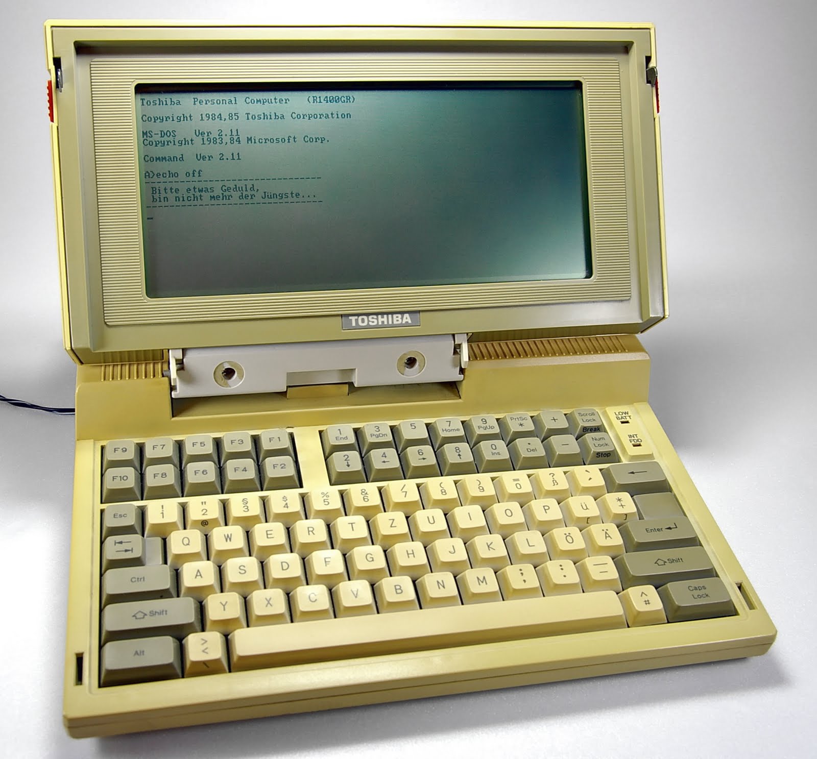
http://inthemoodtoright.blogspot.com/2010/10/worlds-first-laptop.html

The republic of Ireland and the United Kingdom are the only two sovereign states in this image. They are shown in red. Ireland and Great Britain are both islands and are shown in green. England, Scotland, Wales and Northern Ireland are constituent countries of the United Kingdom and are shown in orange. Here, the term “constituent country” is not used in the same way that “country” is usually used; England, Scotland, Wales and Northern Ireland are political entities within the UK, and it is the UK which appears in international bodies such as the United Nations and NATO.
You have the basic idea. There are many other islands in the British Isles which are not shown here. Most of these are politically part of England, Scotland, Wales, Northern Ireland or the republic of Ireland, with the exceptions of the Isle of Man and the Channel Islands, which are British crown dependencies and not part of the UK (or ROI) at all.
The UK’s full name is “the United Kingdom of Great Britain and Northern Ireland”.
“Britain” is not a technically correct term for any political or geographical entity. Nevertheless, “Britain” is in frequent use, and taken to mean either “the UK” or “Great Britain”. This usage is pretty unfair to Northern Ireland whichever way you look at it.
The ROI’s full name is “Ireland” (if you are speaking English) or “Éire” (if you are speaking Irish).
Ireland is popularly referred to as “the Republic of Ireland” in order to distinguish it from the island of Ireland, and the country is indeed a republic, but “the Republic of” is not part of the country’s official name, and I suppose technically this means that the R need not be capitalized.
Citizens of the UK are called “British”. One British person is called a Briton.
Citizens of the ROI are called “Irish”.
Irish citizens are not British citizens. British citizens are not Irish citizens.
There is no such thing as English, Scottish, Welsh or Northern Irish citizenship. English, Scottish, Welsh and Northern Irish people almost always hold British citizenships.
Of course, anybody, living anywhere in the British Isles or the world, can have any ethnicity, and hold any citizenship.
Many people living in Northern Ireland (which is part of the UK) are citizens of the ROI (which is not part of the UK).
Some citizens of the UK living in Northern Ireland (which is part of the UK) classify themselves as Irish-ethnic.
Some people living in Northern Ireland (which is part of the UK) would even like Northern Ireland itself classified as part of the ROI instead of the UK. This is a contentious point.
The ROI is not British. However, the “British Isles” include both the UK and ROI. Irish citizens and Irish-ethnic people hate this, but there is no consensus on what to call it instead. (May I suggest “The British and Irish Isles”?)
England, Wales, Scotland, Northern Ireland and the republic of Ireland frequently field separate teams in such sports as rugby, football (i.e. the World Cup), cricket and so on. Meanwhile, the Irish international rugby team is composed of players chosen from both the ROI and Northern Ireland. This is largely because our various nations have been playing rugby, football and cricket for centuries, whereas the current political arrangement of the British Isles was only established in 1920.
Lastly, to be pedantic, this is actually an Euler diagram, not a Venn diagram.
Taken from qntm.org
